Rendering
Rendering is an extremely time-consuming task. At the same time, it is one that can have significant speedups when there are sufficient resources available. In this section, we experimented different rendering tasks and measured the effective gains.
Rendering an Image
In this experiment, we tested the scalability of the popular raytracer POVRay. This is one of Khepri's rendering backends and, therefore, we used Khepri to generate the following 3D structure containing different materials (metal, glass, etc.):
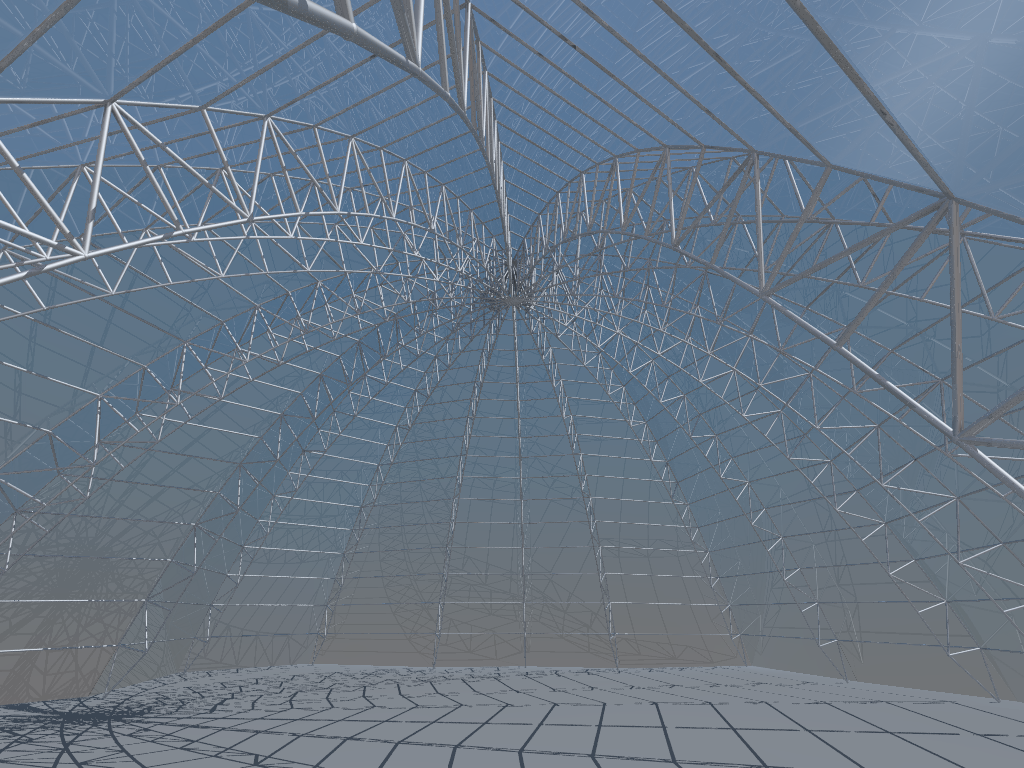
Usually, Khepri handles POVRay without any help from the user but, in this experiment, we did not want to include the time it takes Khepri to generate the information required for POVRay and then to start the process. Therefore, we took the input files generated by Khepri for POVRay and we tested them directly.
We knew that, by default, POVRay uses all available CPUs to divide most of the raytracing process between them. However, we found it difficult to make it use fewer CPUs, even when we specified so on the batch script. We were able to solve the problem by using POVRay's Work_Threads option, which specifies the number of threads that it should use. The corresponding Slurm script looked like this:
#!/bin/bash

#SBATCH --job-name=TestPOVRay
#SBATCH --time=02:00:00
#SBATCH --nodes=1
#SBATCH --ntasks=1
#SBATCH -p <...>
#SBATCH -q <...>

time povray Work_Threads=$SLURM_CPUS_ON_NODE DomeTrussRibs.ini
In this experiment, to avoid fluctuations in the load of the computing node, we decided to repeat the test three times and present the average. First, we attempted to render a 1024 by 768 image. The real time spent for different numbers of threads is the following:

To have another data point, we then decided to change the point of view, while also increasing the size of the image from the previous 1024x768 to 1920x1024. This changes not only the number of pixels, but also the aspect ratio, producing the following image:
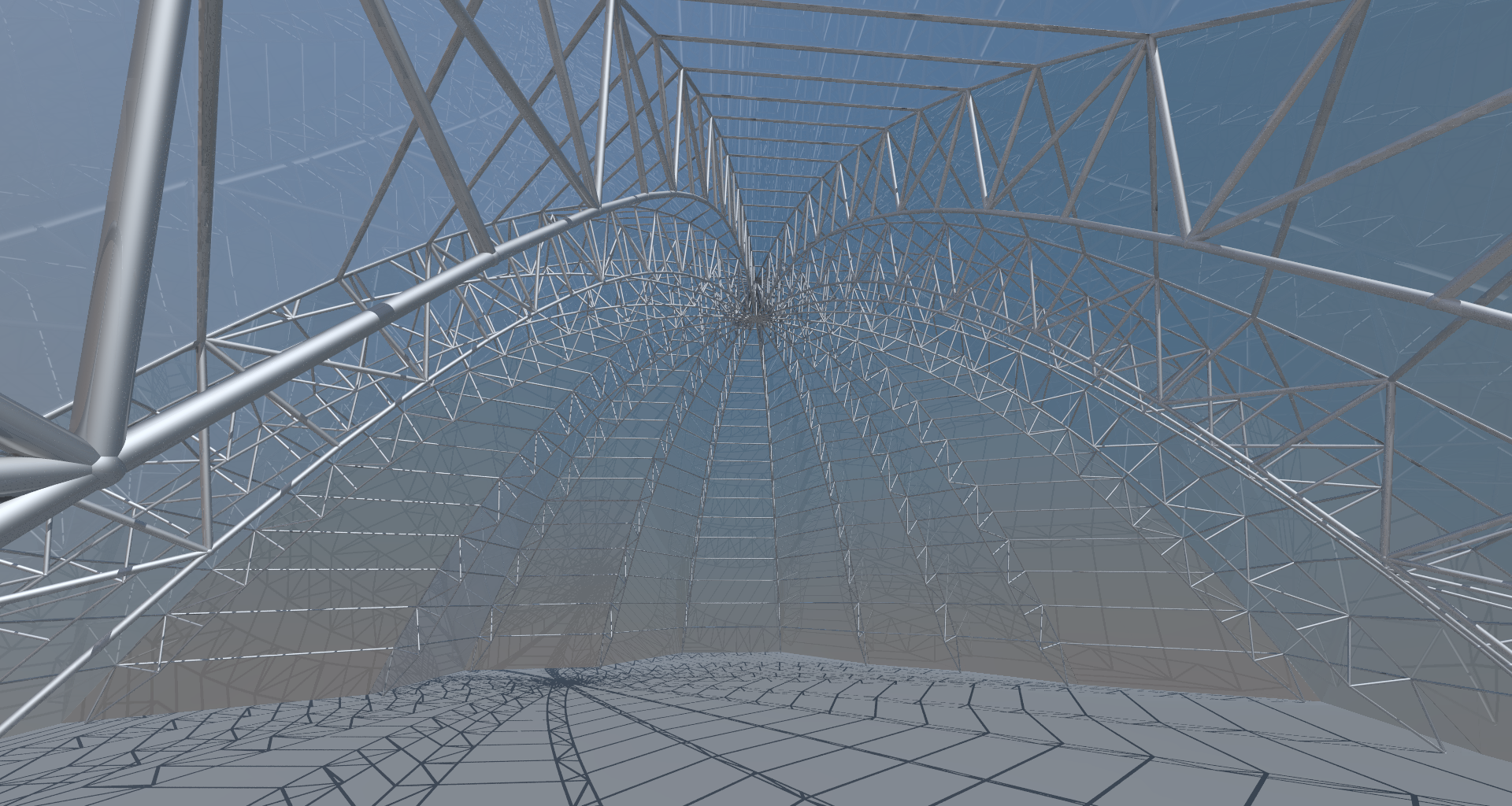
Again, we took the average of three different runs. The result is the following:

Note that there are relevant speedups up to the upper limit of threads. Although it pales in comparison to the initial gains, from 80 threads to 96 threads, there is still a significant reduction from 130.8 seconds to 110.3 seconds.
By analyzing the speedups, we can determine the number of threads that we should use.

As is visible, for the small rendering task, it only pays off to use up to 80 threads, for an almost 40X speedup compared to just one thread. After that, the gains appear to be marginal. In the case of the large rendering task, despite the fluctuations, we were able to reach a speedup of almost 65 and the trend line shows that there are even bigger potential speedups waiting for us. In fact, POVRay can take advantage of 512 threads, so we are still a long way from that limit.
Rendering a Movie
A movie is made of a sequence of images and, therefore, rendering a movie implies rendering multiples images. For smooth visualization, we should use a minimum of 30 frames per second, which means that a short 10-seconds movie requires at least 300 rendered images. If we further assume that the images should be in Full HD, i.e., using 1920x1080 pixels, then it becomes obvious that even a short movie can take a huge amount of time on a normal computer. In the recent past, we did several of these movies and it was not unusual to wait days or weeks for the completion of the rendering process.
As we saw in the previous section, using the Cirrus supercomputer the time needed to render each frame becomes acceptable and thus, it is tempting to just generate all of the needed frames in sequence. This relieves the programmer from having to coordinate multiple processes. The following study of daylight, made of 157 frames at a resolution of 1024x768, was entirely done in 79m36s:
Given that the speedup gets bigger at higher resolutions, we attempted the same experiment but now using 1920x1080 pixels and for a smoother effect, 391 frames:
This time, it took 797m30s, fitting the typical overnight rendering job.
We saw in the previous experiment that POVRay will explore all available threads to render just one frame and, so, there are no more computational resources available that we can use to further speedup the process. If we start more POVRay processes on the computing node, the computing resources will be divided among them and, therefore, we will slowdown all of them. However, the Cirrus supercomputer has multiple computing nodes. This means that, although it might not be possible to speedup up the rendering of one image beyond the 96 threads available in one computing node, it is possible to speedup the rendering of a sequence of images by dividing the sequence among all available computing nodes. In our case, we were allowed to use four computing nodes and, although we did not experiment it because there were other jobs running that made it impossible to reserve all computing nodes for ourselves, it is clear that it would be possible to divide the rendering tasks among the four different computing nodes to achieve a further 4X speedup, allowing the rendering of a Full HD movie to achieve a speedup of 250.
An easier experiment to do is the production of different movies. In this case, there is no need to coordinate the different computing nodes as each one can do a completely separate job. To prove this, we did a study on the different turbidity degrees of the atmosphere. First, we wrote a small Khepri script that would receive the turbidity degree as a command line argument and would generate a 400-frames movie of an animated object that is being viewed by a camera that rotates around it:
using KhepriPOVRay

turbidity=parse(Int, ARGS[1])
realistic_sky(turbidity=turbidity)

render_dir(@__DIR__)
render_size(1920, 1024)

chrome = material(povray=>povray_include("textures.inc", "texture", "Polished_Chrome"))
ground(-5)

start_film("MetalGlassTree$(turbidity)")
nframes = 400
for (rho, phi, z) in zip(division(80, 10, nframes),division(0, 2*pi, nframes),division(0, 40, nframes))
 delete_all_shapes()
 for i in 0:19
   p0 = cyl(23 - i, i, 2*i - 2*sin(4*phi))
   p1 = cyl(23 - i, i + pi, 2*i + 2*sin(4*phi))
   sphere(p0, 2 + 0.5*sin(4*phi), material=chrome)
   sphere(p1, 2 - 0.5*sin(4*phi), material=chrome)
   cylinder(p0, 1, p1, material=material_glass)
 end
 set_view(cyl(rho, phi, z), xyz(0, 0, 30), 20.0)
 save_film_frame()
end
We tested the script using eight different turbidity levels. The following videos illustrate the same animated object rendered under a selection of such levels (more specifically, 2, 4, 6, and 8):
The videos for the eight turbidity levels took, respectively, 94m8.523s, 75m36.726s, 73m30.351s, 73m19.054s, 71m32.826s, 71m23.082s, 70m53.158s, and 70m28.809s. Using just one computing node would entail roughly 10 hours (more exactly, 600m52.529s) but, as we were spreading the different independent jobs among the four computing nodes that we could use, it took around 2h50m (more exactly, 169m42.249s). This result could be improved if we could use more computing nodes: each video could have been generated in a different computing node, and the total computation would have taken around 1h30m (more exactly, 94m8.523s).
For a more architectonic example, here is a study on different materials applied to a building's façade:
The 360 frames in each of the three videos, in total, required 106 minutes to complete. However, by using three different nodes, we could have divided this time, roughly, by three.
We also experimented with the renderings of glass in white or black backgrounds. To that end, we created the following Khepri program, which uses a ratio from 0.1 to 1.0 to affect the radius of each randomly placed sphere:
default_material(material_glass)

ratio = Parameter(0.1)

spheres_in_sphere(p, ri, re, rl, n) =
  if n == 0
    true
  else
    r = random_range(ri, re)
    sphere(p+vsph(r, random_range(0.0, 2*pi), random_range(0.0, pi)), (rl-r)*ratio())
    spheres_in_sphere(p, ri, re, rl, n-1)
  end
To generate the frames, we just iterate, increasing the ratio on each frame, while rotating the spheres:
ground(-6, material(povray=>povray_definition(
  "Ground", "texture",
  "{ pigment { color rgb 1 } finish { reflection 0 ambient 0 }}")))
realistic_sky()
render_size(1080,1080)
render_dir(@__DIR__)
set_view(xyz(9.9307, -93.0178, 63.675), xyz(0.0841, -0.9705, 0.5236), 300)

start_film("RotatingGrowingSpheres")
for ϕ in division(0, 2π, 720)
  delete_all_shapes()
  set_random_seed(12345)
  with(current_cs, cs_from_o_phi(u0(), ϕ), ratio, ϕ/(2π)) do
    spheres_in_sphere(xyz(0, 0, 0), 4.0, 5.0, 5.0, 600)
  end
  save_film_frame()
end
Then just by changing the rgb color of the ground, we generate the two different backgrounds. The results are the following:
The film with white background took 218m15.151s while the one with the black background took 89m36.919s. This is one example where dividing the work among two computing nodes does not provide as much benefit as we would like because one of the videos takes much longer to produce than the other. Nevertheless, it still saves almost one and a half hour in a job that would take five hours to complete, a still significant 30% reduction.
Finally, given that the focus was architecture, we decided to repeat a series of videos that we did in the past, at a time where we spent weeks rendering films that, in some cases, would take one hour for each frame. Given the differences in the available software, it is not possible to exactly replicate the images, as the rendering engine is necessarily different. However, it can give a sense of the trade-offs between speed and image quality.
The first video shows a parametric exploration of the Astana National Library, a project originally designed BIG architects (the video was 'filmed' at Full HD resolution but was reduced to half its size to facilitate viewing):
For another example:
Evolution
We saw that supercomputers can have a dramatic effect on the time needed for rendering tasks. By parallelizing the rendering of a single image through the multi-processing capabilities of a computing node and then parallelizing the rendering of multiple images through the use of multiple computing nodes, it becomes possible to achieve very large speedups.
At the same time, it is relevant to consider that even commodity hardware, nowadays, can efficiently run multiple threads in parallel. This means that the speedups obtained in the previous experiments must be contrasted not with the minimum computing power that the supercomputer can provide but, instead, with the current computing power that is available almost everywhere. In this analysis, the results do not look as good as they seemed. As a reference, using the maximum computing power available on one computing node, i.e., 96 execution threads, we managed to render the 1920x1024 image in an average of 110.3 seconds. For comparison, a 2017 AMD ThreadRipper 1950X workstation providing 16 cores/32 threads renders that same image in 615.5 seconds, which represents a speedup of only 5.6. For an even more depressing comparison, a 2015 Intel 4 cores/8 threads i7-6700K CPU that costs around 250 EUR can render the same image in 1946.4 seconds while doing other useful tasks at the same time. Although the supercomputer gives us a speedup of 17.6, just the CPU costs 18 times more. The ratio cost/performance seems to be, at best, constant.
Despite the cost, the supercomputer does make the rendering task more feasible. We decided to test some additional examples that, in the past, were almost impractical. As a first example, in 2010, the following image, by Prateek Karandikar, took 16 hours and 19 seconds to render on an Intel Pentium 1.8GHz machine with 1GB RAM.

The supercomputer could generate the same image in 51 seconds, which is more than three orders of magnitude faster.
As another example, consider the classical POVRay Hall-of-Fame Pebbles example, which is entirely procedurally generated:
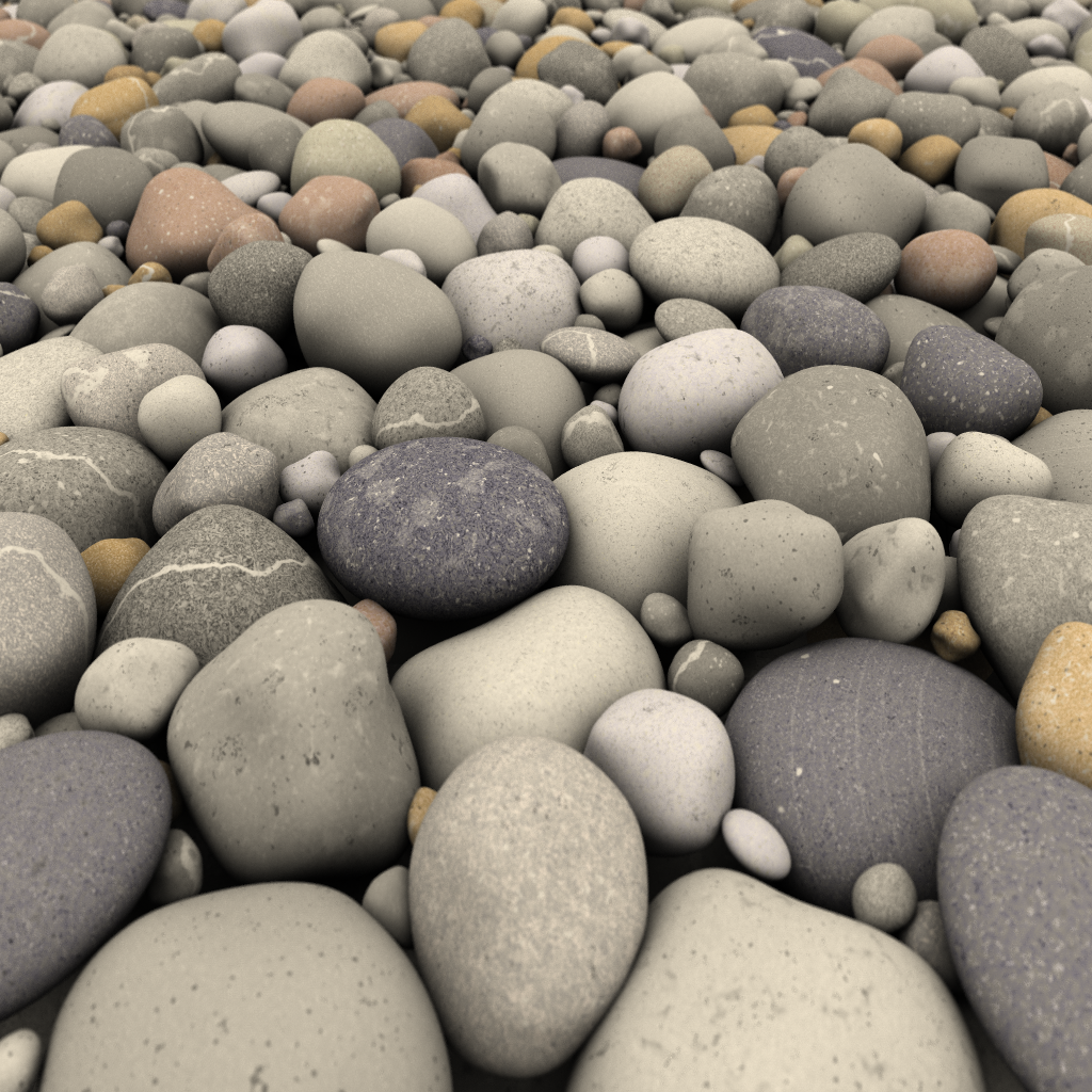
According to its author, this image took 4.5 days to render on an Athlon 5600+. We generated the exact same image on the supercomputer in 2h49m. This is a speedup of almost 40, which opens the door to other ideas. One was to use the exact same POVRay program to do a short movie just by changing the camera's position. The result is not very smooth but it gives an idea of what becomes possible: